Examples

This notebook shows an example of how to use Chopchop.

import matplotlib.pyplot as plt
import numpy as np

from chopchop import InstrumentContext, DefaultTelemetryStrategy, simulate_telemetry

Instrument context

The instrument context contains the information about the instrument and the data that will be used in the Chopchop algorithm, such as the data generation rate, the amount of priority data, or the duration of a telemetry session.

You can initialize a context with default values, or override them with your own values to create a custom scenario.

In the following, we set the data packet loss rate to 10%.

context = InstrumentContext(packet_loss_rate=0.1)

context

InstrumentContext(segment_duration=300.0, session_duration=28800.0, session_interval=86400.0, sc_generation_rate=10980.0, priority_sc_generation_rate=3580.0, generation_rate_margin=0.5, packet_overhead=0.1, downlink_overhead=20000.0, sc2sc_transfer_time=8.3391023799538, sc2ground_transfer_time=166.78204759907604, packet_loss_rate=0.1)

We can print a summary of derived parameters, such as the total data volume to be downloaded during a telemetry session, the required download rate, or the time to download all archived data since the last telemetry session.

context.print_derived_parameters()

Volume of archived data to download per telemetry session: 6423.926 Mbits
Necessary download rate to send all live data in a session: 223.1 kbps
Volume of priority-1 data in one segement: 5316.3 kbits
Download time for one priority-1 data segment: 23.8 s
Number of segments that can be downloaded between priority live segments: 11
Time to download all priority-1 archived data: 1.5 h

Strategy

The strategy is the algorithm that will be used to select the data to download during a telemetry session. For now, we only have the Chopchop strategy, but more strategies will be added in the future.

The default Chopchop strategy is to download the high-priority live data first, and interleave the archived data packets. Lost packets are retransmitted between live packets when all archived data has been downloaded.

strategy = DefaultTelemetryStrategy()

Simulating a telemetry session

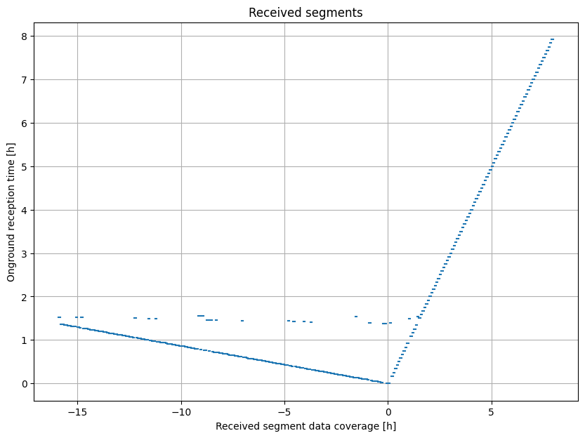
We can now simulate a telemetry session to get a list of received packets, the corresponding data segemnts and reception times, the lost packets, etc.

The TelemetrySimulation instance you get offers many convenience functions to plot the received packets, and the available data segments.

telemetry = simulate_telemetry(strategy, context)

print(f"Number of received packets: {len(telemetry.received_packets)}")
print("First lost packet:", telemetry.lost_packets[:3])

Number of received packets: 287
First lost packet: [(47.66849134510632, DataSegment(-600.0 to -300.0)), (71.50273701765948, DataSegment(-900.0 to -600.0)), (262.17670239808473, DataSegment(-3300.0 to -3000.0))]

telemetry.plot_received_segments()
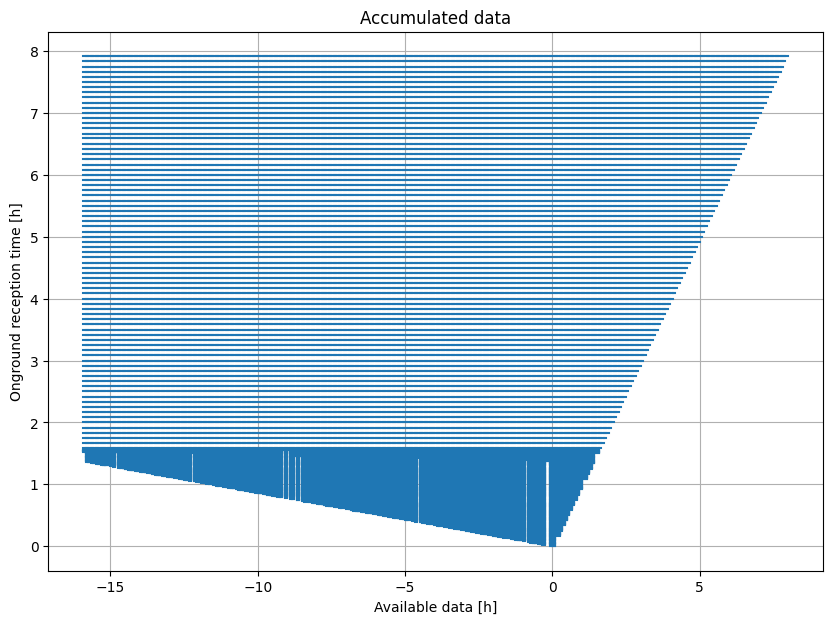
telemetry.plot_accumulated_data()

We can compute masks to select the available data from a continous data array.

data_times = np.arange(-15 * 3600, 10 * 3600)  # s
masks = telemetry.compute_masks(data_times)

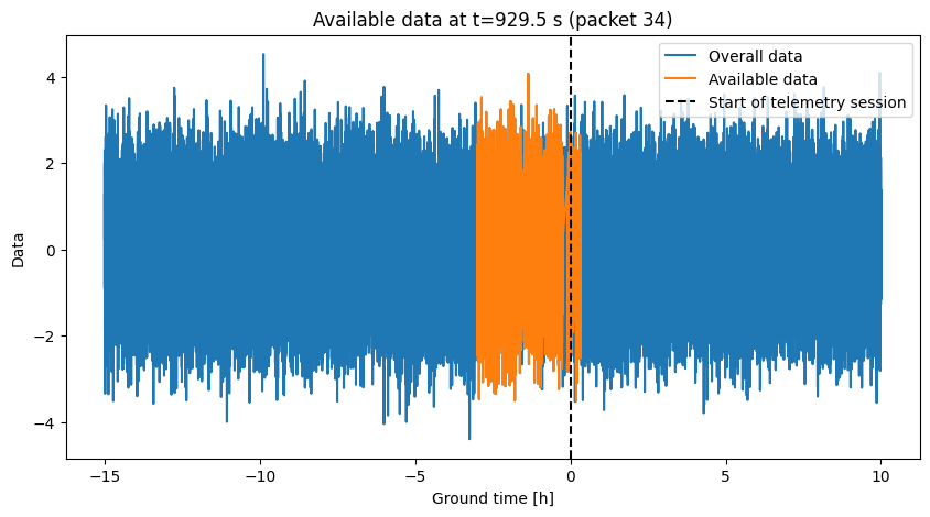
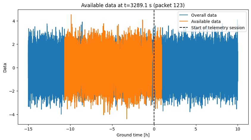
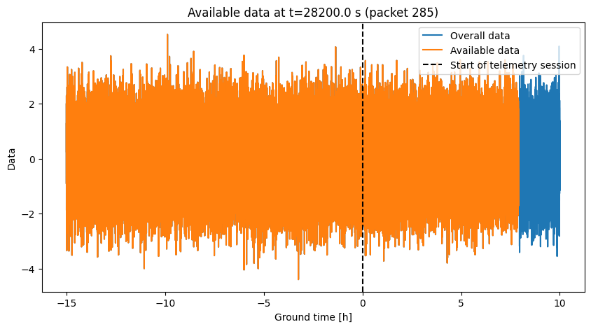
As an example, we plot the available data after the 34th, 123th, and 285th packets have been received.

overall_data = np.random.randn(len(data_times))


def plot_available_data_after_packet(i: int) -> None:
    """Plot the available data after a given packet index."""

    mask = masks[i]
    time = telemetry.reception_times[i]

    plt.figure(figsize=(10, 5))
    plt.plot(data_times / 3600, overall_data, label="Overall data")
    plt.plot(
        data_times[mask] / 3600,
        overall_data[mask],
        label="Available data",
    )
    plt.axvline(0, color="black", linestyle="--", label="Start of telemetry session")
    plt.legend()
    plt.xlabel("Ground time [h]")
    plt.ylabel("Data")
    plt.title(f"Available data at t={time:.1f} s (packet {i})")


plot_available_data_after_packet(34)
plot_available_data_after_packet(123)
plot_available_data_after_packet(285)